Introduction

This tutorial will show you how to build a basic speech recognition network that recognizes simple speech commands. Speech recognition is a subfield of computer science and linguistics that identifies spoken words and converts them into text.

A Basic Understanding of the Techniques Involved

When speech is recorded using a voice recording device like a microphone, it converts physical sound to electrical energy. Then, using an analog-to-digital converter, this is converted to digital data, which can be fed to a neural network or hidden Markov model to convert them to text.

We are going to train such a neural network here, which, after training, will be able to recognize small speech commands.

Speech recognition is also known as:

• Automatic Speech Recognition (ASR)

• Computer Speech Recognition

• Speech to Text (STT)

The steps involved are:

1. Import required libraries

2. Download dataset

3. Data Exploration and Visualization

4. Preprocessing

5. Training

6. Testing

Here is a colab notebook with all of the codes if you want to follow along.

Let us start the implementation.

Step 1: Import Necessary Modules and Dependencies

# import libraries

import os
import IPython
import matplotlib.pyplot as plt
import numpy as np
import tensorflow as tf
from tensorflow.keras import layers
from tensorflow.keras import models

Step 2: Download the Dataset

Download and extract the mini_speech_commands.zip, file containing the smaller Speech Commands datasets.

# Download the dataset

!wget 'http://storage.googleapis.com/download.tensorflow.org/data/mini_speech_commands.zip'
!unzip mini_speech_commands.zip

The dataset's audio clips are stored in eight folders corresponding to each speech command: no, yes,down,go,left, up,right,and stop.

Dataset: TensorFlow recently released the Speech Commands Datasets. It includes 65,000 one-second long utterances of 30 short words by thousands of different people. We will be working with a smaller version of the Speech Commands dataset called mini speech command datasets.

Download the mini Speech Commands dataset and unzip it.

!wget 'http://storage.googleapis.com/download.tensorflow.org/data/mini_speech_commands.zip'
!unzip mini_speech_commands.zip

The dataset's audio clips are stored in eight folders corresponding to each speech command: no yes down go left up right and stop

Now that we have the dataset, let us understand and visualize it.

Step 3: Data Exploration and Visualization

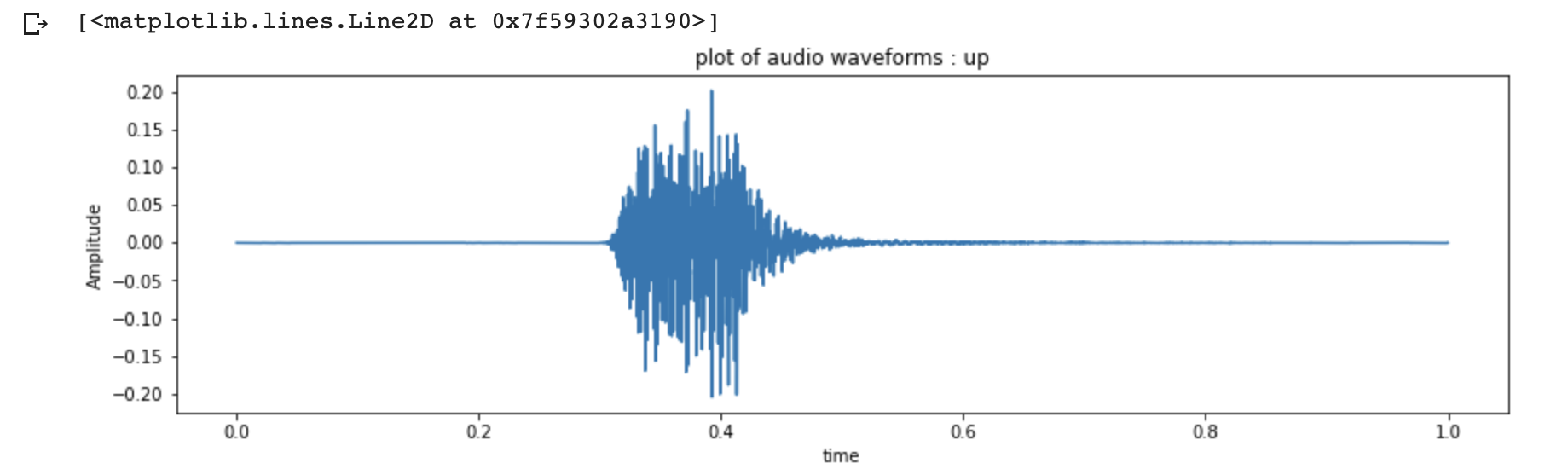
Data Exploration and Visualization is an approach that helps us understand what's in a dataset and the characteristics of the dataset. Let us visualize the audio signal in the time series domain.

#load the data
audio_data_path = '/content/mini_speech_commands/'
samples, sample_rate = librosa.load(audio_data_path+'up/0132a06d_nohash_2.wav', sr = 16000)

#plot waveform 
fig = plt.figure(figsize=(14, 8))
ax1 = fig.add_subplot(211)
ax1.set_title('plot of audio waveforms : up')
ax1.set_xlabel('time')
ax1.set_ylabel('Amplitude')
ax1.plot(np.linspace(0, sample_rate/len(samples), sample_rate), samples)

Here is what the audio looks in a waveform.

To listen to the above command up :

IPython.display.Audio(data=samples, rate=8000)

Check the list of commands for which we will be training our speech recognition model. These audio clips are stored in eight folders corresponding to each speech command: no, yes, down, go, left, up, right, and stop.

commands_list = np.array(tf.io.gfile.listdir(str(audio_data_path)))
commands_list = commands_list[commands_list != 'README.md']
print('Commands_list:', commands_list)

Remove unnecessary files:

!rm '/content/mini_speech_commands/README.md'

Let us plot a bar graph to understand the number of recordings for each of the eight voice commands:

labels=os.listdir(audio_data_path)

no_of_recordings=[]
for label in labels:
  waves = [f for f in os.listdir(audio_data_path + '/'+ label) if f.endswith('.wav')]
  no_of_recordings.append(len(waves))

#plot
plt.figure(figsize=(30,5))
index = np.arange(len(labels))
plt.bar(index, no_of_recordings)
plt.xlabel('Commands', fontsize=12)
plt.ylabel('No of recordings', fontsize=12)
plt.xticks(index, labels, fontsize=15, rotation=60)
plt.title('No. of recordings for each command')
plt.show()

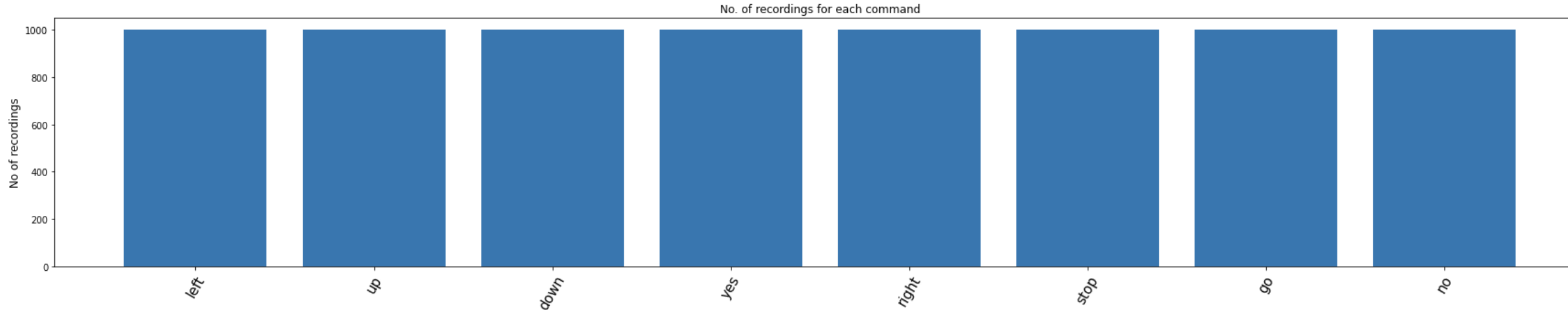
As we can see, we have almost the same number of recordings for each command.

Step 4: Preprocessing

Let us define these preprocessing steps in the code snippet below:

# Let us define these preprocessing steps in the below code snippet:

train_audio_path = '/content/mini_speech_commands'

all_wave = []
all_label = []
for label in labels:
    print(label)
    waves = [f for f in os.listdir(train_audio_path + '/'+ label) if f.endswith('.wav')]
    for wav in waves:
        samples, sample_rate = librosa.load(train_audio_path + '/' + label + '/' + wav, sr = 16000)
        samples = librosa.resample(samples, sample_rate, 8000)
        if(len(samples)== 8000) : 
            all_wave.append(samples)
            all_label.append(label)

Convert the output labels to integer encoded labels and then to a one-hot vector since it is a multi-classification problem. Then reshape the 2D array to 3D since the input to the conv1d must be a 3D array:

# Convert the output labels to integer encoded:

from sklearn.preprocessing import LabelEncoder
le = LabelEncoder()
y=le.fit_transform(all_label)
classes= list(le.classes_)

from keras.utils import np_utils
y=np_utils.to_categorical(y, num_classes=len(labels))

all_wave = np.array(all_wave).reshape(-1,8000,1)

Step 5: Training

Train test split - train test split is a model validation procedure that allows you to simulate how a model would perform on new/unseen data. We are doing an 80:20 split of data for training and testing.

from sklearn.model_selection import train_test_split
x_tr, x_val, y_tr, y_val = train_test_split(np.array(all_wave),np.array(y),stratify=y,test_size = 0.2,random_state=777,shuffle=True)

Create a model and compile it. Now, we define a model:

# define a model

from keras.layers import Dense, Dropout, Flatten, Conv1D, Input, MaxPooling1D
from keras.models import Model
from keras.callbacks import EarlyStopping, ModelCheckpoint
from keras import backend as K
K.clear_session()

inputs = Input(shape=(8000,1))

#First Conv1D layer
my_model = Conv1D(8,13, padding='valid', activation='relu', strides=1)(inputs)
my_model = MaxPooling1D(3)(my_model)
my_model = Dropout(0.3)(my_model)

#Second Conv1D layer
my_model = Conv1D(16, 11, padding='valid', activation='relu', strides=1)(my_model)
my_model = MaxPooling1D(3)(my_model)
my_model = Dropout(0.3)(my_model)

#Third Conv1D layer
my_model = Conv1D(32, 9, padding='valid', activation='relu', strides=1)(my_model)
my_model = MaxPooling1D(3)(my_model)
my_model = Dropout(0.3)(my_model)

#Fourth Conv1D layer
my_model = Conv1D(64, 7, padding='valid', activation='relu', strides=1)(my_model)
my_model = MaxPooling1D(3)(my_model)
my_model = Dropout(0.3)(my_model)

#Flatten layer
my_model = Flatten()(my_model)

#Dense Layer 1
my_model = Dense(256, activation='relu')(my_model)
my_model = Dropout(0.3)(my_model)

#Dense Layer 2
my_model = Dense(128, activation='relu')(my_model)
my_model = Dropout(0.3)(my_model)

outputs = Dense(len(labels), activation='softmax')(my_model)

model = Model(inputs, outputs)
model.summary()


# Define the loss function to be categorical cross-entropy since it is a multi-classification problem:



model.compile(loss='categorical_crossentropy',optimizer='adam',metrics=['accuracy'])

Define callbacks:

es = EarlyStopping(monitor='val_loss', mode='min', verbose=1, patience=10, min_delta=0.0001) 
mc = ModelCheckpoint('best_model.hdf5', monitor='val_accuracy', verbose=1, save_best_only=True, mode='max')

Start the training:

history=model.fit(x_tr, y_tr ,epochs=100, callbacks=[es,mc], batch_size=32, validation_data=(x_val,y_val))

Plot the training loss vs validation loss:

from matplotlib import pyplot
pyplot.plot(history.history['loss'], label='train')
pyplot.plot(history.history['val_loss'], label='test')
pyplot.legend()
pyplot.show()

Step 6: Testing and Prediction

Now, we have a trained model. We need to load it and use it to predict our commands.

Load the model for prediction:

#Loading the best model

from keras.models import load_model
model=load_model('best_model.hdf5')


#Define the function that predicts text for the given audio:



def predict(audio):
    prob=model.predict(audio.reshape(1,8000,1))
    index=np.argmax(prob[0])
    return classes[index]

Start predicting:

import IPython.display as ipd

import random
index=random.randint(0,len(x_val)-1)
samples=x_val[index].ravel()
print("Audio:",classes[np.argmax(y_val[index])])
ipd.Audio(samples, rate=8000)

You can always create your own dataset with creative ways like clap sounds and whistles or your own custom words and train your model to recognize them.

Demo Video

You can check out the demo video for this experiment here.

Parting Thoughts

We just completed a tutorial on building a speech recognition system! Here is a quick recap:

We began by exploring the dataset, giving us a good feel for what is inside. Then, we prepped the data, converting it into a format suitable for training. After a train-test split, we designed a Conv1D neural network for the task.

By following these steps, we have laid the foundation for a speech recognition system. With further tweaks and your own data, you can expand its capabilities. Keep exploring the world of speech recognition!

---

This article was written by Priyamvada, Software Engineer, for the GeekyAnts blog.