This is a step-by-step tutorial on training object detection models on a custom dataset.

What is Object Detection?

Object Detection (OD) is a computer vision technique that allows us to identify and locate objects in digital images/videos. It is basically a combination of localizing objects in images/videos and classifying them into respective classes. Object detection is used extensively in many interesting areas of work and study, such as

• Security

• ANPR(automatic number plate detection)

• Crowd counting

• Self-driving cars

• Anomaly detection

• Medical field

Object detection is commonly confused with image recognition. Image recognition assigns a label to an image. On the other hand object detection draws a box around the recognized object. The model predicts where each object is and what label should be applied. In that way, object detection provides more information about an image than recognition.

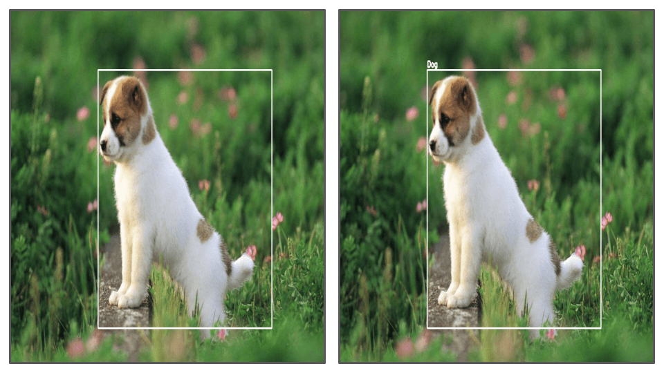
Image Recognition vs Object Detection, Respectively.

Here, we are going to use YOLO family of object detectors, specifically YOLOv3.

What is YOLO?

YOLO (You Only Look Once) is a state-of-the-art, real-time object detection system. Since its inception, it has evolved from v1 to YOLOvX to this date. To Know more about YOLO versions, you can refer here. We are going to focus on yolov3 for this tutorial.

• For the purpose of this tutorial, we will be using Google Colab to train on a sample dataset we have provided. Follow the steps below.

Required libraries :

• Python 3.5 or higher

• Tensorflow

• OpenCV

This tutorial is divided into 3 main steps:

• Collecting and preparing custom data

• Training

• Testing

Let us get started. Notebook for the code is provided here, you can follow along with the code. We will now look into the steps needed.

Step 1 : Collecting and Preparing Custom Data

Gathering the data

For custom object detection, you need some data to train and test the model. You can either download an already labeled public data set or create your own data set.

Some great sites to get public data sets are:

• Kaggle

• Roboflow

• Google Image Dataset

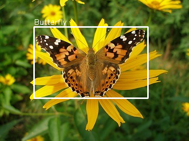
To create your own dataset, you can download images from the internet or take pictures yourself. You can decide the number of classes you want you want to train on. Here, we are training our model for one class - butterfly. For this, I have created a sample dataset by downloading 100 images of a butterfly from here. The entire dataset has ten categories and 832 images, but for now, we are using 100 images for creating a sample dataset. Next, we need to annotate these images.

Note : If you are using already labeled dataset, make sure to convert them in yolo format and you can skip the annotation step. For this, take a look here. YOLO format is explained below.

Annotation

Next, we need to annotate these images, there are many tools available for this:

• LabelImg

• MakeSense.AI

• VGG image annotator

• LabelMe

• Scalable

• RectLabel

There is no single standard format when it comes to image annotation. Some of the commonly used annotation formats are COCO, YOLO, and Pascal VOC. For getting image annotations in YOLO format, https://github.com/tzutalin/labelImg is preferred as it is easy to install and use. For installing, check out https://github.com/tzutalin/labelImg. If you choose to use this tool for annotations, make sure to change the output format to YOLO.

If you want to know more about different Image Annotation Types, you can check out this.

YOLO Format

In YOLO labeling format, a .txt file with the same name is created for each image file in the same directory. Each .txt file contains the annotations for the corresponding image file, that is, object class, object coordinates, height, and width. For each object, a new line is created. Below is an example of annotation in YOLO format :

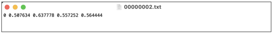
You can save all the annotations fine in the same folder as the images and name the folder images.

Step 2 : Prerequisites for Training

1. Mount Drive and Get Images Folder

For training, we are going to take advantage of the free GPU offered by Google Colab.

• Create a new folder in Google Drive called yolo_custom_training

• Zip the images folder and upload the zipped file to the empty directory yolo_custom_training , on the drive

• Go to Google Colab, create a new notebook, and name it YOLO_custom_training_notebook

• Mount Google Drive and give permission when asked to access Google Drive

# mount google drive
from google.colab import drive
drive.mount('/content/gdrive')
!ln -s /content/gdrive/My\ Drive/ /mydrive
!ls /mydrive

• Unzip the images folder

# unzip images folder
!unzip /content/gdrive/MyDrive/yolo_custom_training/images.zip -d /content/gdrive/MyDrive/yolo_custom_training

Next, we are going to install dependencies.

2. Clone the Darknet

You Only Look Once (YOLO) utilizes darknet for real-time object detection, ImageNet classification, recurrent neural networks (RNNs), and many others.

Darknet is an open-source neural network framework written in C and CUDA. It is fast, easy to install, and supports CPU and GPU computation. Advanced implementations of deep neural networks can be done using Darknet.

First, we need to clone the repo and then compile it. Before compiling, in the case of GPU, you need to make some changes in Makefile to utilize GPU acceleration. You need to change GPU = 1, CUDNN =1, OPENCV = 1. If using CPU, leave it at 0. Since we are using Google Colab, which gives us free access to GPU, we are going to make these changes.

• Clone the Darknet

!git clone 'https://github.com/AlexeyAB/darknet.git' '/content/gdrive/MyDrive/yolo_custom_training/darknet'

• Compile Darknet using NVIDIA GPU, make changes in makefile, GPU,CUDNN,OPENCV=1

# change makefile to have GPU and OPENCV enabled
%cd /content/gdrive/MyDrive/yolo_custom_training/darknet
!sed -i 's/OPENCV=0/OPENCV=1/' Makefile
!sed -i 's/GPU=0/GPU=1/' Makefile
!sed -i 's/CUDNN=0/CUDNN=1/' Makefile
!make clean
!make

3. Configure Darknet Network for Training YOLO V3 - Update CFG File for Training

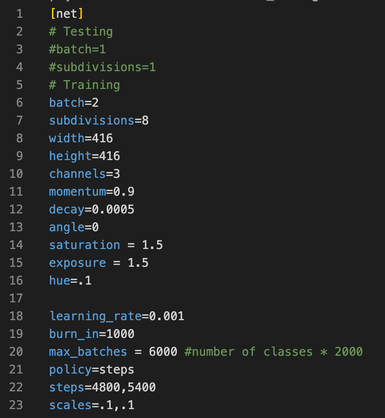
Once you have the Darknet folder, you need to make some changes in the CFG file which contains details about your training and testing like batch size, hyperparameters etc.

• For training, we will make a copy of the CFG file and make required changes

!cp cfg/yolov3.cfg cfg/yolov3_custom_training.cfg

• Change line batch to [batch=2]

• Change line subdivisions to [subdivisions=8]

• Change line max_batches to (classes*2000, but not less than the number of training images, and not less than 6000), i.e. [max_batches=6000] if you train for three classes

• Change line steps to 80% and 90% of max_batches. For example, [steps=4800,5400]

• For training, comment batch and subdivision for testing i.e. lines 3 and 4

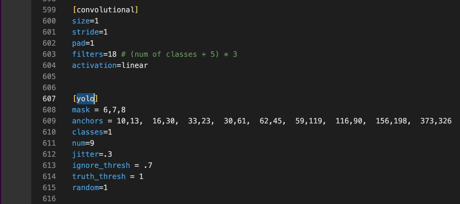
• Change line classes=1 to your number of objects in each of 3 [yolo] layers

• Change [filters=255] to filters=(classes + 5)x3 in the 3 [convolutional] before each [yolo] layer, keep in mind that it only has to be the last [convolutional] before each of the [yolo] layers. So if classes=1then should be filters=18. If classes=2then write filters=21

• To make changes in CFG file, you can either download the file, make the following changes on local and upload it on drive at /content/gdrive/MyDrive/yolo_custom_training/cfg/yolov3_custom_training.cfg,

or in Colab, we can use the following command line commands:

!sed -i 's/batch=1/batch=2/' cfg/yolov3_custom_training.cfg
!sed -i 's/subdivisions=1/subdivisions=8/' cfg/yolov3_custom_training.cfg
!sed -i 's/max_batches = 500200/max_batches = 6000/' cfg/yolov3_custom_training.cfg
!sed -i '610 s@classes=80@classes=1@' cfg/yolov3_custom_training.cfg
!sed -i '696 s@classes=80@classes=1@' cfg/yolov3_custom_training.cfg
!sed -i '783 s@classes=80@classes=1@' cfg/yolov3_custom_training.cfg
!sed -i '603 s@filters=255@filters=18@' cfg/yolov3_custom_training.cfg
!sed -i '689 s@filters=255@filters=18@' cfg/yolov3_custom_training.cfg
!sed -i '776 s@filters=255@filters=18@' cfg/yolov3_custom_training.cfg

• For training , we need to comment the testing batch size and subdivision and similarly while testing, we need to comment training parameters.

# For trianing
!sed -i '3 s@batch=1@# batch=1@' cfg/yolov3_custom_training.cfg
!sed -i '4 s@subdivisions=1@# subdivisions=1@' cfg/yolov3_custom_training.cfg
!sed -i '6 s@# batch=64@batch=64@' cfg/yolov3_custom_training.cfg
!sed -i '7 s@# subdivisions=16@subdivisions=16@' cfg/yolov3_custom_training.cfg

4. Setup the Data Config Files

path_data.data contains the details of the dataset you want to train your model on. The file looks like this. We will create the required files one by one.

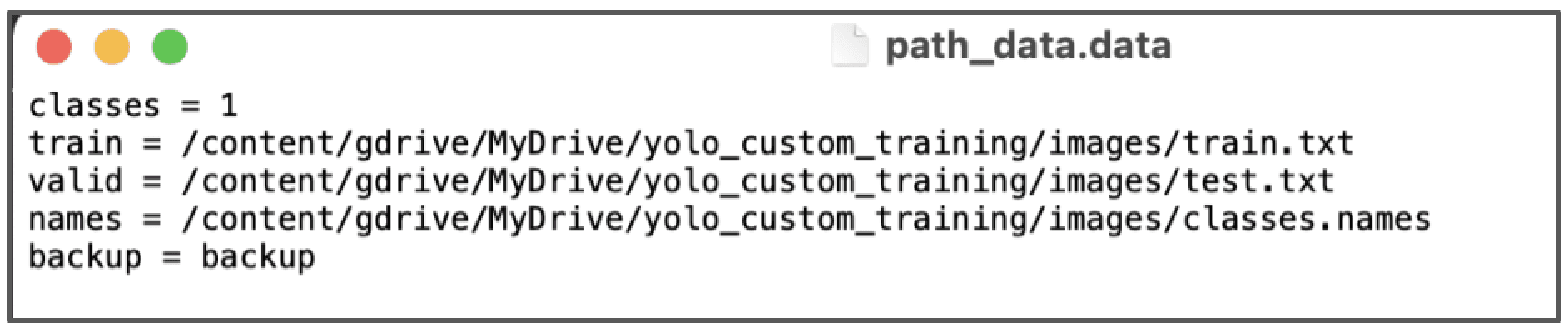
1. train, test, and val: Locations of train, test, and validation images

2. classes: Number of classes in the dataset

3. names: path of names of the classes in the dataset(classes.names file). The index of the classes in this list would be used as an identifier for the class names in the code

4. backup: Folder path in which the weights will be saved after training

Let us create these files.

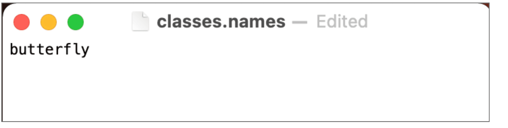
• Create classes.names files

Create classes.names files that contains objects names - each in new line. We can create one using classes.txt file created during annotations file.

images_dir = '/content/gdrive/MyDrive/yolo_custom_training/images'

# starting counter for classes
c = 0

# Creating file classes.names from classes.txt

with open(images_dir + '/' + 'classes.names', 'w') as classes, \
     open(images_dir + '/' + 'classes.txt', 'r') as txt:

    for line in txt:
        classes.write(line)

        c += 1

or create it manually.

• Create path_data.data

# Creating file path_data.data

with open(images_dir + '/' + 'path_data.data', 'w') as content:

    content.write('classes = ' + str(c) + '\n')

    # Location of the train.txt file
    content.write('train = ' + images_dir + '/' + 'train.txt' + '\n')

    # Location of the test.txt file
    content.write('valid = ' + images_dir + '/' + 'test.txt' + '\n')

    # Location of the classes.names file
    content.write('names = ' + images_dir + '/' + 'classes.names' + '\n')

    # Location where to save weights
    content.write('backup = backup')

• Create backup folder in /content/gdrive/MyDrive/yolo_custom_training/images/

!mkdir /content/gdrive/MyDrive/yolo_custom_training/images/backup

• Create file train.txt and test.txt

Create file train.txt and test.txt in directory /content/gdrive/MyDrive/yolo_custom_training/images\ , with filenames of your images, each filename in new line, with path relative to darknet.exe, for example containing:

# Creating file train.txt and writing 85% of lines in it

p = [os.path.join(images_dir,f) for f in os.listdir(images_dir) if f.endswith('.png')]

os.chdir(images_dir)

# Slicing first 15% of elements for test
p_test = p[:int(len(p) * 0.15)]

# Deleting from initial list first 15% of elements
p = p[int(len(p) * 0.15):]
p = '\n'.join(p)

# Creating file train.txt and writing 85% of lines in it
with open('train.txt', 'w') as train_txt:
    # Going through all elements of the list
    for e in p:
        # Writing current path at the end of the file
        train_txt.write(e)

# Creating file test.txt and writing 15% of lines in it
with open('test.txt', 'w') as test_txt:
    # Going through all elements of the list
    for e in p_test:
        # Writing current path at the end of the file
        test_txt.write(e)

5. Weights

We are going to use transfer learning here. For this, we are going to use a pre-trained model called darknet53.conv.74, trained in various classes. Now, you must create a new folder called custom_weights and place the pre-trained model in it.

 !wget -P '/content/gdrive/MyDrive/yolo_custom_training/custom_weight' 'https://pjreddie.com/media/files/darknet53.conv.74'

6. Start the Training

Start training by using the command line:

%cd /content/gdrive/MyDrive/yolo_custom_training

!darknet/darknet detector train custom_data/labelled_data.data darknet/cfg/yolov3_custom.cfg custom_weight/darknet53.conv.74 -dont_show

Step 3 : Testing the Model

After training, the weights will be saved in backup folder that we created earlier. We will be using yolov3_custom_last.weights for testing. You can either download the weights to your local and continue from there, or use Colab.

• Changes in the CFG file

  • For testing, we need to comment on the training parameters in .cfg file by commenting lines 6 and 7 and uncommenting lines 3 and 4.

# For testing
!sed -i '3 s@# batch=64@batch=1@' cfg/yolov3_custom_training.cfg
!sed -i '4 s@# subdivisions=16@subdivisions=1@' cfg/yolov3_custom_training.cfg
!sed -i '6 s@batch=64@#batch=64@' cfg/yolov3_custom_training.cfg
!sed -i '7 s@subdivisions=16@#subdivisions=16@' cfg/yolov3_custom_training.cfg

• Load the model and classes and weights

  • We first read the network model saved in Darknet model files using Opencv’s readNetFromDarknet() function. It requires two parameters, path to the .cfg file and path to the .weights file with the learned network.

import numpy as np
import time
import cv2

INPUT_FILE='/00000021.jpg'
LABELS_FILE='/content/gdrive/MyDrive/yolo_custom_training/images/path_data.data'
CONFIG_FILE='/content/gdrive/MyDrive/yolo_custom_training/darknet/cfg/yolov3_custom.cfg'
WEIGHTS_FILE='/content/gdrive/MyDrive/yolo_custom_training/backup/yolov3_custom_last.weights'
CONFIDENCE_THRESHOLD=0.5

classes = open(LABELS_FILE).read().strip().split("\n")

net = cv2.dnn.readNetFromDarknet(CONFIG_FILE, WEIGHTS_FILE)

• Read the input image and process it for darknet

  • then, we read the input image and its height and width, on which we will make the prediction.

image = cv2.imread(INPUT_FILE)
(H, W) = image.shape[:2]

• Now we have the image in RGB format that has a shape of width*height*channels, but YOLO Net takes images in a different format, so we need to convert it into the required format before feeding it to the network. For this, we use cv2.dnn.blobFromImage(). We are going to feed this blob to our YOLO network.

blob = cv2.dnn.blobFromImage(image, 1 / 255.0, (416, 416),
    swapRB=True, crop=False)
net.setInput(blob)
start = time.time()
layerOutputs = net.forward(ln)
end = time.time()

print("[INFO] YOLO took {:.6f} seconds".format(end - start))

• Determine only the output layer names that we need from YOLO.

# determine only the *output* layer names that we need from YOLO
ln = net.getLayerNames()
ln = [ln[i-1] for i in net.getUnconnectedOutLayers()]

• Predict and draw the predicted boxes.

  Draw a box around the object.

  boxes = []
  confidences = []
  classIDs = []

  for output in layerOutputs:
      for detection in output:
          scores = detection[5:]
          classID = np.argmax(scores)
          confidence = scores[classID]

          if confidence > CONFIDENCE_THRESHOLD:
              # scale the bounding box coordinates back relative to the size of the image
              box = detection[0:4] * np.array([W, H, W, H])
              (centerX, centerY, width, height) = box.astype("int")

              # derive top and and left corner of the bounding box
              x = int(centerX - (width / 2))
              y = int(centerY - (height / 2))

              # update our list of bounding box coordinates, confidences,and class IDs
              boxes.append([x, y, int(width), int(height)])
              confidences.append(float(confidence))
              classIDs.append(classID)

  # apply non-maxima suppression to suppress weak, overlapping bounding boxes
  idxs = cv2.dnn.NMSBoxes(boxes, confidences, CONFIDENCE_THRESHOLD,
      CONFIDENCE_THRESHOLD)

  COLORS = np.random.randint(0, 255, size=(len(classes), 3),
      dtype="uint8")
  if len(idxs) > 0:
      for i in idxs.flatten():
          (x, y) = (boxes[i][0], boxes[i][1])
          (w, h) = (boxes[i][2], boxes[i][3])

          color = [int(c) for c in COLORS[classIDs[i]]]

          cv2.rectangle(image, (x, y), (x + w, y + h), color, 2)
          text = "{}: {:.4f}".format(classes[classIDs[i]], confidences[i])
          cv2.putText(image, text, (x, y - 5), cv2.FONT_HERSHEY_SIMPLEX,
              0.5, color, 2)

  # show the output image
  cv2.imwrite("/content/gdrive/MyDrive/yolo_custom_training/output.png", image)

• You will get the results image with bounding box saved as output.png in /content/gdrive/MyDrive/yolo_custom_training/output.png

Here is the entire code for prediction :

import numpy as np
import time
import cv2

input_file='/Users/priyamvada./Documents/custom_training/images_rookie/00000021.jpg'
labels_file='/Users/priyamvada./Documents/custom_training/images_rookie/path_data.data'
cfg_file='/Users/priyamvada./Documents/custom_training/darknet/cfg/yolov3_custom.cfg'
weights='/Users/priyamvada./Documents/custom_training/yolov3_custom_last.weights'
CONFIDENCE_THRESHOLD=0.3

classes = open(labels_file).read().strip().split("\n")

np.random.seed(4)

net = cv2.dnn.readNetFromDarknet(CONFIG_FILE, WEIGHTS_FILE)

image = cv2.imread(INPUT_FILE)
(H, W) = image.shape[:2]

# determine only the *output* layer names that we need from YOLO
ln = net.getLayerNames()
ln = [ln[i-1] for i in net.getUnconnectedOutLayers()]

blob = cv2.dnn.blobFromImage(image, 1 / 255.0, (416, 416),
    swapRB=True, crop=False)
net.setInput(blob)
start = time.time()
layerOutputs = net.forward(ln)
end = time.time()

print("[INFO] YOLO took {:.6f} seconds".format(end - start))

boxes = []
confidences = []
classIDs = []

for output in layerOutputs:
    for detection in output:
        scores = detection[5:]
        classID = np.argmax(scores)
        confidence = scores[classID]


        if confidence > CONFIDENCE_THRESHOLD:
            # scale the bounding box coordinates back relative to the size of the image
            box = detection[0:4] * np.array([W, H, W, H])
            (centerX, centerY, width, height) = box.astype("int")

            # derive top and and left corner of the bounding box
            x = int(centerX - (width / 2))
            y = int(centerY - (height / 2))

            # update our list of bounding box coordinates, confidences,and class IDs
            boxes.append([x, y, int(width), int(height)])
            confidences.append(float(confidence))
            classIDs.append(classID)

# apply non-maxima suppression to suppress weak, overlapping bounding boxes
idxs = cv2.dnn.NMSBoxes(boxes, confidences, CONFIDENCE_THRESHOLD,
    CONFIDENCE_THRESHOLD)

COLORS = np.random.randint(0, 255, size=(len(classes), 3),
    dtype="uint8")
if len(idxs) > 0:
    for i in idxs.flatten():
        (x, y) = (boxes[i][0], boxes[i][1])
        (w, h) = (boxes[i][2], boxes[i][3])

        color = [int(c) for c in COLORS[classIDs[i]]]

        cv2.rectangle(image, (x, y), (x + w, y + h), color, 2)
        text = "{}: {:.4f}".format(classes[classIDs[i]], confidences[i])
        cv2.putText(image, text, (x, y - 5), cv2.FONT_HERSHEY_SIMPLEX,
            0.5, color, 2)

# show the output image
cv2.imwrite("/Users/priyamvada./Documents/custom_training/images_rookie/example.png", image)

Output Video

Check out this link for a look at the output video.

Conclusion

This comprehensive tutorial offers a detailed and accessible guide to training custom object detection models using the YOLOv3 architecture. By leveraging the state-of-the-art YOLOv3, you can effectively identify and locate objects in images or videos. By following the steps discussed, you can harness the potential of custom object detection models tailored to their specific datasets and applications, ushering in a new era of accuracy and efficiency in object recognition technology.

---

This article was written by Priyamvada, Software Engineer, for the GeekyAnts blog.